Contours
The cxroots module allows the user to specify four different types of contours which are all subclasses of Contour:
- class cxroots.contour.Contour(segments: list[ComplexPathType])[source]
A base class for contours in the complex plane.
- central_point
The point at the center of the contour.
- Type:
complex
- area
The surface area of the contour.
- Type:
float
- __call__(t: float) complex[source]
- __call__(t: ndarray[tuple[int, ...], dtype[floating]]) ndarray[tuple[int, ...], dtype[complexfloating]]
The point on the contour corresponding the value of the parameter t.
- Parameters:
t (float) – A real number \(0\leq t \leq 1\) which parameterises the contour.
- Returns:
A point on the contour.
- Return type:
complex
Example
>>> from cxroots import Circle
>>> c = Circle(0,1) # Circle |z|=1 parameterised by e^{it}
>>> c(0.25)
(6.123233995736766e-17+1j)
>>> c(0) == c(1)
True
- abstract contains(z: complex) bool
True if the point z is within the contour, false otherwise
- count_roots(f: AnalyticFunc, df: AnalyticFunc | None = None, int_abs_tol: float = 0.07, integer_tol: float = 0.1, div_min: int = 3, div_max: int = 15, int_method: Literal['quad', 'romb'] = 'quad') int
For a function of one complex variable, f(z), which is analytic in and within the contour C, return the number of zeros (counting multiplicities) within the contour
- distance(z: complex) float[source]
The distance from the point z in the complex plane to the nearest point on the contour.
- Parameters:
z (complex) – The point from which to measure the distance to the closest point on the contour to z.
- Returns:
The distance from z to the point on the contour which is closest to z.
- Return type:
float
- integrate(f: AnalyticFunc, abs_tol: float = 1.49e-08, rel_tol: float = 1.49e-08, int_method: Literal['quad'] = 'quad') complex[source]
Integrate the function f along the path.
\[\oint_C f(z) dz\]The value of the integral is cached and will be reused if the method is called with same arguments.
- Parameters:
f (function) – A function of a single complex variable.
abs_tol (float, optional) – The absolute tolerance for the integration.
rel_tol (float, optional) – The realative tolerance for the integration.
int_method ({'quad'}, optional) – If ‘quad’ then
scipy.integrate.quad()is used to compute the integral.
- Returns:
The integral of the function f along the path.
- Return type:
complex
- plot(num_points: int = 100, linecolor: str | tuple[float, float, float] | tuple[float, float, float, float] = 'C0', linestyle: str = '-') None[source]
Uses matplotlib to plot, but not show, the path as a 2D plot in the Complex plane.
- Parameters:
num_points (int, optional) – The number of points to use when plotting the path.
linecolor (optional) – The colour of the plotted path, passed to the
matplotlib.pyplot.plot()function as the keyword argument of ‘color’. See the matplotlib tutorial on specifying colours.linestyle (str, optional) – The line style of the plotted path, passed to the
matplotlib.pyplot.plot()function as the keyword argument of ‘linestyle’. The default corresponds to a solid line. Seematplotlib.lines.Line2D.set_linestyle()for other acceptable arguments.
- show(save_file: str | None = None, **plot_kwargs) None[source]
Shows the contour as a 2D plot in the complex plane. Requires Matplotlib.
- Parameters:
save_file (str (optional)) – If given then the plot will be saved to disk with name ‘save_file’. If save_file=None the plot is shown on-screen.
**plot_kwargs – Key word arguments are as in
plot().
- subdivisions(axis: str = 'alternating') Generator[tuple[Contour, ...], None, None][source]
A generator for possible subdivisions of the contour.
- Parameters:
axis (str, 'alternating' or any element of self.axis_names.) – The axis along which the line subdividing the contour is a constant (eg. subdividing a circle along the radial axis will give an outer annulus and an inner circle). If alternating then the dividing axis will always be different to the dividing axis used to create the contour which is now being divided.
- Yields:
tuple – A tuple with two contours which subdivide the original contour.
Circle
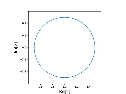
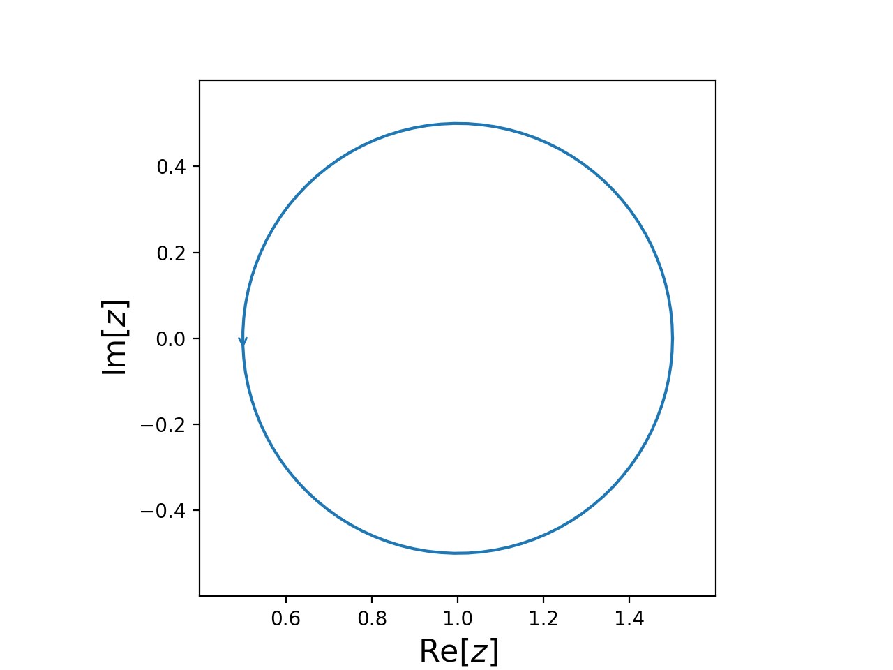
- class cxroots.Circle(center: complex, radius: float)[source]
A positively oriented circle in the complex plane.
- Parameters:
center (complex) – The center of the circle.
radius (float) – The radius of the circle.
Examples
from cxroots import Circle
circle = Circle(center=1, radius=0.5)
circle.show()
(
Source code,png,hires.png,pdf)
Rectangle
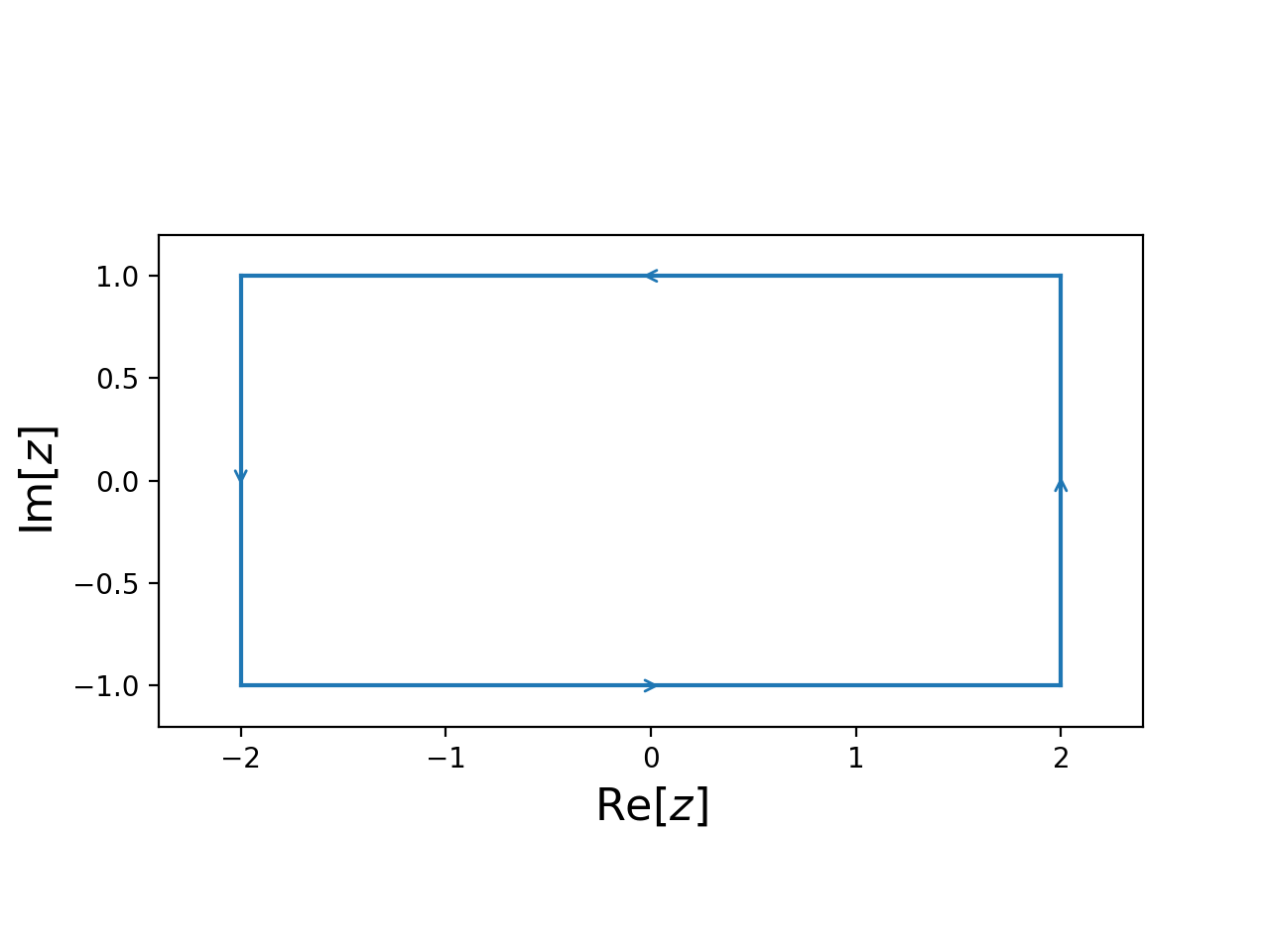
- class cxroots.Rectangle(x_range: tuple[float, float], y_range: tuple[float, float])[source]
A positively oriented rectangle in the complex plane.
- Parameters:
x_range (tuple) – Tuple of length two giving the range of the rectangle along the real axis.
y_range (tuple) – Tuple of length two giving the range of the rectangle along the imaginary axis.
Examples
from cxroots import Rectangle
rect = Rectangle(x_range=(-2, 2), y_range=(-1, 1))
rect.show()
(
Source code,png,hires.png,pdf)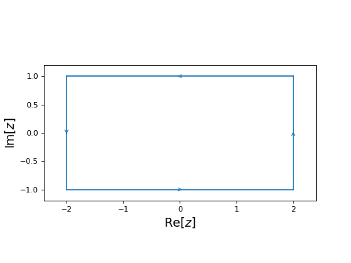
Annulus
- class cxroots.Annulus(center: complex, radii: tuple[float, float])[source]
An annulus in the complex plane with the outer circle positively oriented and the inner circle negatively oriented.
- Parameters:
center (complex) – The center of the annulus in the complex plane.
radii (tuple) – A tuple of length two of the form (inner_radius, outer_radius).
Examples
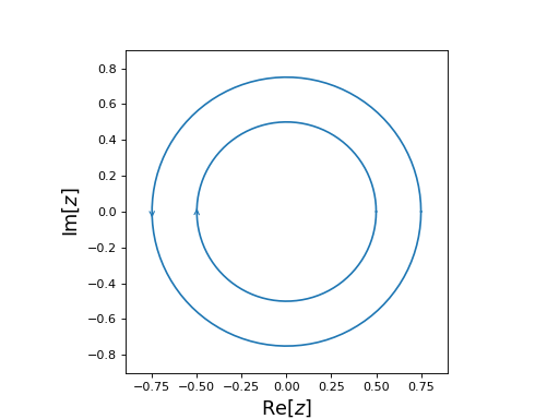
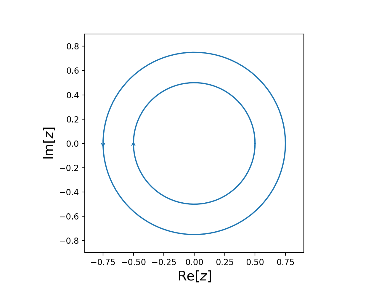
from cxroots import Annulus
annulus = Annulus(center=0, radii=(0.5,0.75))
annulus.show()
(
Source code,png,hires.png,pdf)
Annulus Sector
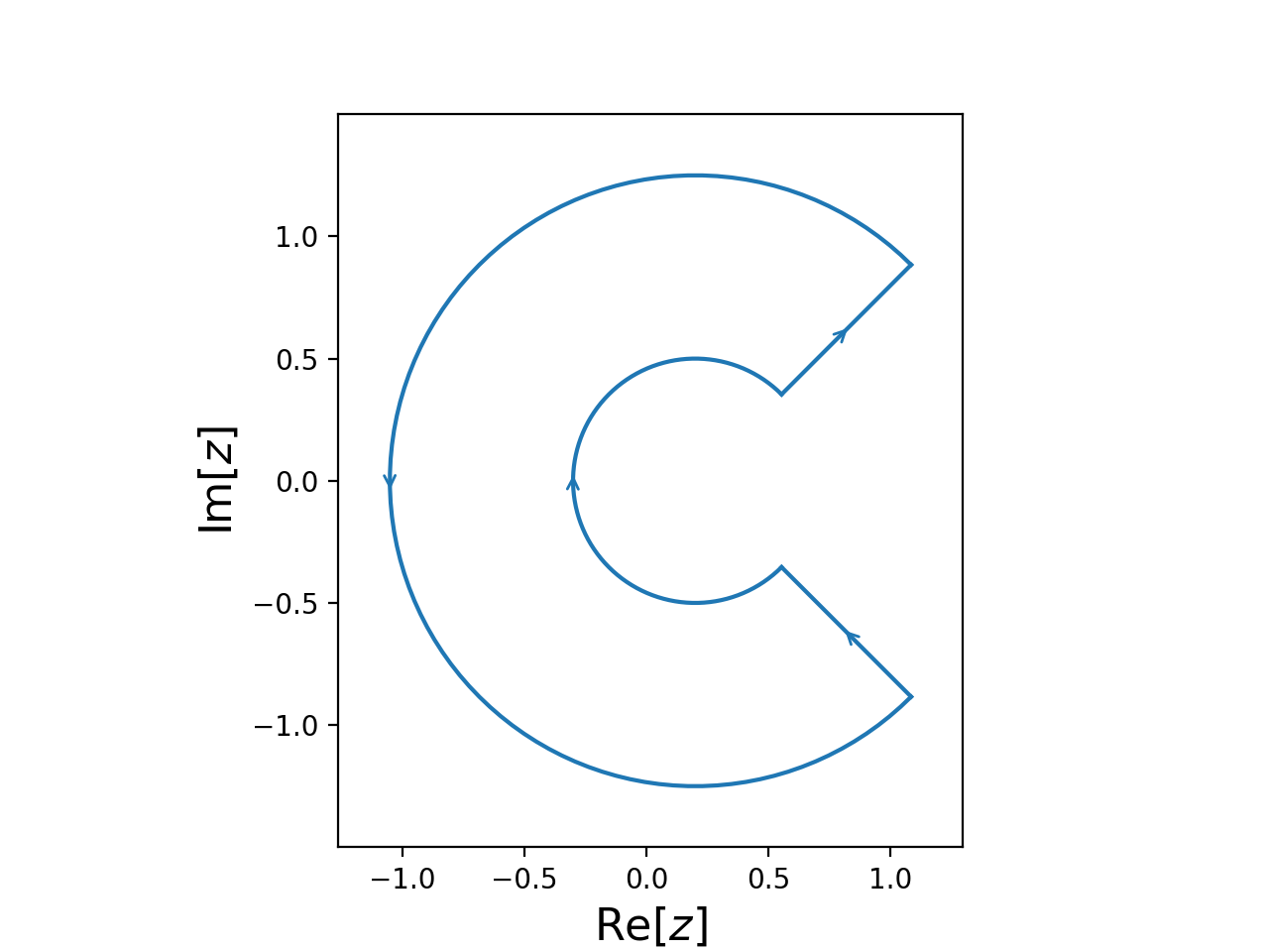
- class cxroots.AnnulusSector(center: complex, radii: tuple[float, float], phi_range: tuple[float, float])[source]
A sector of an annulus in the complex plane.
- Parameters:
center (complex) – The center of the annulus sector.
radii (tuple) – Tuple of length two of the form (inner_radius, outer_radius)
phi_range (tuple) – Tuple of length two of the form (phi0, phi1). The segment of the contour containing inner and outer circular arcs will be joined, counter clockwise from phi0 to phi1.
Examples
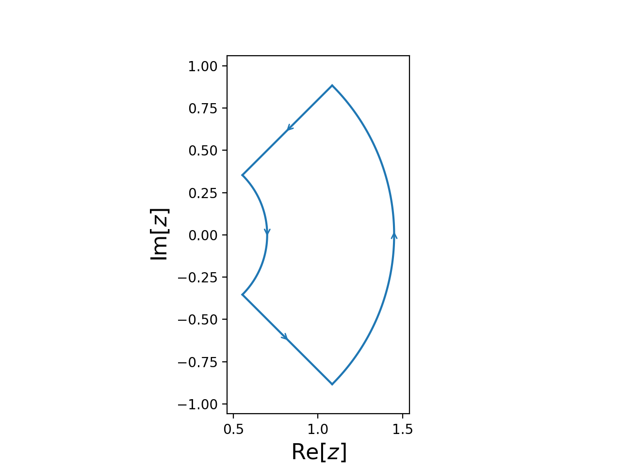
from numpy import pi
from cxroots import AnnulusSector
annulusSector = AnnulusSector(
    center=0.2, radii=(0.5, 1.25), phi_range=(-pi/4, pi/4)
)
annulusSector.show()
(
Source code,png,hires.png,pdf)
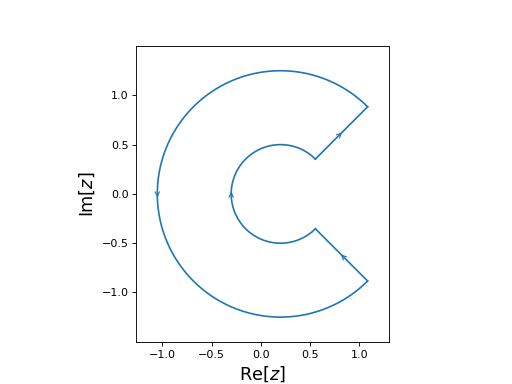
from numpy import pi
from cxroots import AnnulusSector
annulusSector = AnnulusSector(
    center=0.2, radii=(0.5, 1.25), phi_range=(pi/4, -pi/4)
)
annulusSector.show()
(
Source code,png,hires.png,pdf)